Kalman Filter
Hello. I hope you are doing well. Today we will walk through explanation and derivation of famous Kalman Filter (KF).
Gaussian Filters
All the filters that are based on Gaussian filter is usually called Gaussian filters. Gaussian filters mainly work with multivariate gaussian distribution. Pdf of multivariate gaussian distribution can be get by this equation.
$$ p(x) = det(2\pi \Sigma)^{-\frac{1}{2}} \exp(-\frac{1}{2}(x-\mu)^T \Sigma^{-1}(x-\mu))$$
In the place of standard deviation, as in one dimensional gaussian distributio, here, we have \(\Sigma\) covariance matrix which quadratic matriz and has n x n shape where n is the size of x vector. Furthermore, the mean \(\mu\) is mean vector of xs.
According to the parameterization Gaussian filters have two discrete types:
- Moments parameterization (Parameterization of Gaussian filter using Σ and μ)
- Canonical parameterization(natural parameterization).
Kalman filter
Kalman filter(KF) is a moments parameterization kind of Gaussian Filter which is special form of Bayes Filter. So KF obeys Bayesian Filter equation.
$$bel(x_t) = \eta p(z_t | x_t) \int P(x_t | x_{t-1}, u_t) bel(x_{t-1}) d(x_{t-1})$$
Similar to Bayesian Filter it also finds the likelihood of current state based on all the actions that we have performed so far and all the observations we have collected so far. If you recall ,the bayesian filter, we used Markov assumption to state that a) current state only depends on previous estimate and current action. b) current observation only depends on current estimate.
The system of KF assumes these properties:
- The state transition must be linear:
- Measurement equation must also be linear.
- Initial belief must be normally distributed
- \[bel(x_0) = p(x_0) = det(2\pi \Sigma_0)^{-\frac{1}{2}} \exp(-\frac{1}{2}(x_0-\mu_0)^T \Sigma_0^{-1}(x_0-\mu_0))\]
Now lets define the system that KF uses.
Let’s say you have a robot or something like that with noisy sensor, and you want to track its position or some value considering the previous estimate and current action. As well as that, you may want to correct the estimation of the position or some other value based on current observation so that errors get attenuated as much as possible.
- Then you have to estimate its mean every time based on previous estimate and change it according to current observation.
System transition can be obtained using this equation.
$$x_t = A_t x_{t-1} + B_t u_t + \varepsilon_t$$
\(x_t \epsilon R^n\) is state vector which stores the values we want to track.
\(x_{t-1} \epsilon R^n\) is previous state vector.
\(u_t \epsilon R^m\) is action vector which defines the physics of the model. For example if we have an acceleration then we can define it in this vector.
\(A_t \epsilon R^{nxn}\) is state mapping matrix which linearly map the previous state so that new estimate is obtained. For example if we hae x coordinate and \(v_x\) speed then we can add ,assuming the time unit as 1, \(v_x\) to x by using this matrix.
\(B_t \epsilon R^{nxm}\) is here to map current action so that specific action gets added to specific state variable.
\(\varepsilon_t\) is state transition noise.
Observation equation can be obtained using this equation.
$$z_t = C_t x_t + \delta_t$$
\(z_t \epsilon R^n\) is observation vector which stores sensor measurements or any other noisy value that we need to track. This equation is just an assumption that sensor observation is just an actual value plus some added noise.
\(\delta_t\) is measurement noise
The process of Kalman Filer
**this image is captured from the book Probabilistic Robotics (Sebastian Thrun, Wolfram Burgard, Dieter Fox).
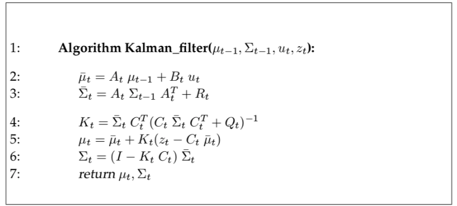
This process can be described as two processes:
- we first predicting new state (mean) and covariance (std) in line 2,3.
- Then we are updating them based on current observation in lines 4,5,6.
The belief of current state is \(bel(x_t)\) is gaussian and its mean is our current state \(\mu \epsilon R^n\) and its covariance is our systems covariance \(\Sigma \epsilon R^{nxn}\).
Here, \(\overline{\mu_t}\) indicates current prior mean estimate and \(\overline{\Sigma}\) is current prior (predicted) covariance.
\(R_t \epsilon R^{nxn}\) is the covariance matrix of state noise \(\varepsilon_t\)
\(K_t \epsilon R^{nxn}\) is kalman gain which defines how much part of the current innovation (difference between current observation prediction and actual observation) \(z_t - C_t\mu_t\) should be used to update the current estimate prediction \(\overline{\mu}\) to get posterior (updated/corrected) mean estimate \(\mu\).
\(\Sigma \epsilon R^{nxn}\) is the posterior (corrected/updated) state covariance matrix.
The main concept of KF is updating the mean and covariance of the distribution so that observation noise is attenuated.
Note that initial state mean and covariance matrices will be given manually and can be arbitrary.
Kalman Filter derivation
Since, the KF system is gaussian we can write its pdf using multivariate gaussian which has mean and covariance.
$$ p(x) = det(2\pi \Sigma)^{-\frac{1}{2}} \exp(-\frac{1}{2}(x-\mu)^T \Sigma^{-1}(x-\mu))$$
Lets now define \(p(x_t|u_t, x_{t-1}\) in its gaussian form. KF assumes that state transition is linear and its pdf is normal gaussian.For state transition probability we have mean value \(\mu_t = A_t x_t + B_t u_t\) and covariance \(R_t\). If we plug them into original gaussian distribution equatin above we will get this.
$$ p(x_t|u_t, x_{t-1}) = det(2\pi R_t)^{-\frac{1}{2}} \exp(-\frac{1}{2}(x_t-A_t x_{t-1} - B_t u_t)^T R_t^{-1}(x_t-A_t x_{t-1} - B_t u_t))$$
Lets now do the same with observation likelihood prediction \(p(z_t|x_t)\). KF also asumes that observation equation is linear and its pdf is gaussian.Thus,here, the mean of the distribution is \(C_t x_t\) and covariance is measurment noise’s \(\delta_t\) ‘s covariance \(Q_t\). Hence, the pdf of observation model becomes like this.
$$ p(z_t|x_t) = det(2\pi Q_t)^{-\frac{1}{2}} \exp(-\frac{1}{2}(z_t-C_t x_t)^T Q_t^{-1}(z_t-C_t x_t))$$
Since the KF is recursive as Bayesian Filter(BF) we need to define it’s termination postiion which is initial position. KF assumes that the initial belief is gaussian and is defined with this equation.
$$ bel(x_0) = p(x_0) = det(2\pi \Sigma_0)^{-\frac{1}{2}} \exp(-\frac{1}{2}(x_0-\mu_0)^T \Sigma_0^{-1}(x_0-\mu_0))$$
Since KF is special case of BF lets try to derive it using BF equation.
$$bel(x_t) = \eta p(z_t | x_t) \int P(x_t | x_{t-1}, u_t) bel(x_{t-1}) d(x_{t-1})$$
BF is divided into two parts prediction and correction.The full BF above gives us the posterior or the corrected belief. Let us now consider only on prediction which is the integral part of the BF equation.
$$\overline{bel}(x_t) = \int P(x_t | x_{t-1}, u_t) bel(x_{t-1}) d(x_{t-1})$$
| This is also called prior belief — the belief we have before seeing current observation. KF assumes that the \(bel(x_t)\) is gaussian so $$P(x_t | x_{t-1}$$ must be gaussian. Integral of the gaussian is also gaussian so we have no problem with that. |
Let us now write this prior belief or prediction in its gaussian form.
$$\overline{bel}(x_t) = \eta \int \exp(-\frac{1}{2}(x_t-A_t x_{t-1} - B_t u_t)^T R_t^{-1}(x_t-A_t x_{t-1} - B_t u_t)) \exp(-\frac{1}{2}(x_{t-1}-\mu_{t-1})^T \Sigma_t^{-1}(x_{t-1}-\mu_{t-1})) d(x_{t-1})$$
We can write two exponent form as one exponent
$$\overline{bel}(x_t) = \eta \int \exp(-L_t) d(x_{t-1})$$
And, its’ arguments will be summed:
$$L_t = \frac{1}{2}(x_t-A_t x_{t-1} - B_t u_t)^T R_t^{-1}(x_t-A_t x_{t-1} - B_t u_t) + \frac{1}{2}(x_{t-1}-\mu_{t-1})^T \Sigma_t^{-1}(x_{t-1}-\mu_{t-1})$$
As you have noticed Lt is quadratic in xt, xt-1.
Now we need to reorder the terms in the \(L_t\) so that we get two equations in which first one should only depend on \(xt_1\) and second term on \(x_t\). (Here, in first equation, we should keep the terms with xt so that after few modification they must disappear and only variable must be \(xt_1\)).
$$L_t = L_t(x_{t-1}, x_t) + L_t(x_t)$$
Since the integral is calculated on \(x_{t-1}\) and second equation does not have that variable we can bring the exponent of second equation \(L_t(x_t)\) out of integral.
$$\overline{bel}(x_t) = \eta \int \exp(- L_t(x_{t-1}, x_t) - L_t(x_t)) d(x_{t-1}) $$ $$=\eta exp(L_t(x_t)) \int \exp(- L_t(x_{t-1}, x_t)) d(x_{t-1}) $$
The remaining integral is just a integral on \(x_{t-1}\), so the result of the integral will be constant and we can subsume it into constant term ղ.
$$\overline{bel}(x_t)= \eta exp(L_t(x_t)) $$
In order to find that decomposition we need to perform these:
-
We need to find \(L_t(x_{t-1}, x_t)\) quadratic in \(x_{t-1}\) (There is also \(x_t\) but we will eliminate it during the process)
-
Lets take first two derivatives of \(L_t\) on \(x_t\)
$$L_t = \frac{1}{2}(x_t-A_t x_{t-1} - B_t u_t)^T R_t^{-1}(x_t-A_t x_{t-1} - B_t u_t) + \frac{1}{2}(x_{t-1}-\mu_{t-1})^T \Sigma_t^{-1}(x_{t-1}-\mu_{t-1}) $$ $$\frac{\delta L_t}{\delta x_{t-1}} = -A_t^T R_t^T (x_t - A_t x_{t-1} - B_t u_t) + \Sigma_{t-1}^{-1} (x_{t-1}-\mu_{t-1}) $$ $$\frac{\delta^2 L_t}{\delta x_{t-1}^2} = A_t^T R_t^T A_t + \Sigma_{t-1}^{-1} $$ Lets make some assumptins: $$\frac{\delta L_t}{\delta x_{t-1}} = \frac{\delta L_t(x_{t-1},x_t)}{\delta x_{t-1}} $$ $$\frac{\delta^2 L_t}{\delta x_{t-1}^2} = \frac{\delta^2 L_t(x_{t-1},x_t)}{\delta x_{t-1}^2} $$
Since \(L_t(x_{t-1},x_t)\) is quadratic on \(x_{t-1}\) it resembles gaussian distribution equation. So, lets make that distribution. Minimum of that function is located on mean, we can find it by equalizing first derivative to zero. Second derivative gives inverse of the covariance of this gaussian.
it’s covariance:
$$ \frac{\delta^2 L_t(x_{t-1},x_t)}{\delta x_{t-1}^2} = A_t^T R_t^T A_t + \Sigma_{t-1}^{-1} = \Phi_t^{-1}$$
Let us now find its’ mean
$$\frac{\delta L_t}{\delta x_{t-1}} = -A_t^T R_t^T (x_t - A_t x_{t-1} - B_t u_t) + \Sigma_{t-1}^{-1} (x_{t-1}-\mu_{t-1}) $$
$$A_t^T R_t^T (x_t - A_t x_{t-1} - B_t u_t) = \Sigma_{t-1}^{-1} (x_{t-1}-\mu_{t-1})$$
$$A_t^T R_t^T (x_t - B_t u_t ) -A_t^T R_t^T A_t x_{t-1} = \Sigma_{t-1}^{-1} x_{t-1} - \Sigma_{t-1}^{-1}\mu_{t-1}$$
$$ A_t^T R_t^T A_t x_{t-1} +\Sigma_{t-1}^{-1} x_{t-1} = A_t^T R_t^T (x_t - B_t u_t ) + \Sigma_{t-1}^{-1}\mu_{t-1}$$
$$ (A_t^T R_t^T A_t +\Sigma_{t-1}^{-1}) x_{t-1} = A_t^T R_t^T (x_t - B_t u_t ) + \Sigma_{t-1}^{-1}\mu_{t-1}$$
$$ \Phi_t^{-1} x_{t-1} = A_t^T R_t^T (x_t - B_t u_t ) + \Sigma_{t-1}^{-1}\mu_{t-1}$$
Finally the mean:
$$ x_{t-1} = \Phi_t[A_t^T R_t^T (x_t - B_t u_t ) + \Sigma_{t-1}^{-1}\mu_{t-1}]$$
Now let us define the function \(L_t(x_{t-1}, x_t)\).
$$ L_t(x_{t-1}, x_t) = \frac{1}{2}(x_{t-1} -\Phi_t[A_t^T R_t^T (x_t - B_t u_t ) + \Sigma_{t-1}^{-1}\mu_{t-1}] )^T \Phi_t^{-1} (x_{t-1} -\Phi_t[A_t^T R_t^T (x_t - B_t u_t ) + \Sigma_{t-1}^{-1}\mu_{t-1}] ) $$
This is the only function that resembles argument of negative exponent of the this multivariate normal distribution:
$$ det(2\pi \Phi)^{-\frac{1}{2}} \exp(-L_t(x_{t-1}, x_t))$$
We now that integral (surface) of pdf of normal distribution equal to 1
$$ \int det(2\pi \Phi)^{-\frac{1}{2}} \exp(-L_t(x_{t-1}, x_t)) = 1$$
If we move the constant term on the other side of the equation above we will get
$$ \int \exp(-L_t(x_{t-1}, x_t)) = det(2\pi \Phi)^{\frac{1}{2}} $$
If we replace the integral with that constant \(det(2\pi \Phi)^{\frac{1}{2}}\) and subsume this into constant value ղ, we will get the proof of this equation which we stated earlier. Just be attentive that constant terms are not the same after we absorbed integral into old ղ.
$$\overline{bel}(x_t)= \eta exp(L_t(x_t)) \int \exp(- L_t(x_{t-1}, x_t)) d(x_{t-1})= \eta exp(L_t(x_t)) $$
Now, we can find \(L_t(x_t)\) easily by just subtracting \(L_t(x_{t-1},x_t)\) from \(L_t\).
$$L_t(x_t) = L_t - L_t(x_{t-1}, x_t) = \frac{1}{2}(x_t-A_t x_{t-1} - B_t u_t)^T R_t^{-1}(x_t-A_t x_{t-1} - B_t u_t) + \frac{1}{2}(x_{t-1}-\mu_{t-1})^T \Sigma_t^{-1}(x_{t-1}-\mu_{t-1}) - $$ $$ \frac{1}{2}(x_{t-1} -\Phi_t[A_t^T R_t^T (x_t - B_t u_t ) + \Sigma_{t-1}^{-1}\mu_{t-1}] )^T \Phi_t^{-1} (x_{t-1} -\Phi_t[A_t^T R_t^T (x_t - B_t u_t ) + \Sigma_{t-1}^{-1}\mu_{t-1}] )$$
Lets substitute \(\Phi_t\)’s original form \(\Phi_t^{-1} = A_t^T R_t^T A_t + \Sigma_{t-1}^{-1}\) into the equation above and multiply everything.
$$L_t(x_t) = \underline{\underline{\frac{1}{2} x_{t-1}^T A_t^T R_t^{-1} A_t x_{t-1}}}- \underline{x_{t-1}^T A_t^T R_t^{-1}(x_t - B_t u_t)}$$ $$+\frac{1}{2}(x_t - B_t u_t)^T R_t^{-1}(x_t - B_t u_t)$$ $$+\underline{\underline{ x_{t-1}^T \Sigma_{t-1}^{-1} x_{t-1} }} - \underline{x_{t-1}^T \Sigma_{t-1}^{-1} \mu_{t-1}} + \frac{1}{2} \mu_{t-1}^T \Sigma_{t-1}^{-1} \mu_{t-1} $$ $$\underline{\underline{ -\frac{1}{2} x_{t-1}^T (A_t^T R_t^{-1} A_t +\Sigma_{t-1}^{-1} ) x_{t-1} }} $$ $$+x_{t-1}^T[A_t^T R_t^{-1} (x_t - B_t u_t ) + \Sigma_{t-1}^{-1}\mu_{t-1}] $$ $$ -\frac{1}{2} [A_t^T R_t^{-1} (x_t - B_t u_t ) + \Sigma_{t-1}^{-1}\mu_{t-1}]^T (A_t^T R_t^{-1} A_t + \Sigma_{t-1}^{-1})^{-1} [A_t^T R_t^{-1} (x_t - B_t u_t ) + \Sigma_{t-1}^{-1}\mu_{t-1}]$$
In above equation every part of the equation that has \(x_{t-1}\) is underlined or double underlined if there are two of them. You can confirm that all terms that contain \(x_{t-1}\) cancel out. This is because the quadratic function we chose was really the solution . Finally we will reach to our \(L_t(x_t)\).
$$ L_t(x_t) = + \frac{1}{2} (x_t - B_t u_t )^T R_t^{-1} (x_t - B_t u_t ) + \frac{1}{2} \mu_{t-1}^T \Sigma_{t-1}^{-1} \mu_{t-1}$$ $$ -\frac{1}{2} [A_t^T R_t^{-1} (x_t - B_t u_t ) + \Sigma_{t-1}^{-1}\mu_{t-1}]^T (A_t^T R_t^{-1} A_t + \Sigma_{t-1}^{-1})^{-1} [A_t^T R_t^{-1} (x_t - B_t u_t ) + \Sigma_{t-1}^{-1}\mu_{t-1}]$$
The book Probabilistic Robotics (Sebastian Thrun Wolfram Burgard Dieter Fox) have intorduced Inversion Lemma .

\(Lt(xt)\) is quadratic on xt so it satisfies the normal distribution form and mean and covariance of the distribution is at its’ minimum. So we will take first derivative and equalize it to zero to obtain the mean. And for covariance it’s second derivative.
$$ \frac{\delta L_t(x_t)}{\delta x_t} = R_t^{-1}(x_t - B_t u_t ) - R_t^{-1} A_t (A_t^T R_t^{-1} A_t +\Sigma_{t-1}^{-1})^{-1} [A_t^T R_t^{-1} (x_t - B_t u_t ) + \Sigma_{t-1}^{-1}\mu_{t-1}] $$ $$ =[R_t^{-1} - R_t^{-1} A_t (A_t^T R_t^{-1} A_t +\Sigma_{t-1}^{-1})^{-1} A_t^T R_t^{-1}] (x_t - B_t u_t ) $$ $$-R_t^{-1} A_t (A_t^T R_t^{-1} A_t + \Sigma_{t-1}^{-1})^{-1} \Sigma_{t-1}^{-1} \mu_{t-1} $$
The inversions inside the equation above suits inversion dilemma.
$$ R_t^{-1} - R_t^{-1} A_t (A_t^T R_t^{-1} A_t + \Sigma_{t-1}^{-1})^{-1} A_t^T R_t^{-1} = (R_t + A_t \Sigma_{t-1}^{-1} A_t^T) ^{-1} $$
So we greatly simplify the equation of first derivation of \(Lt(xt)\).
$$ \frac{\delta L_t(x_t)}{\delta x_t} = (R_t + A_t \Sigma_{t-1}^{-1} A_t^T) ^{-1} (x_t - B_t u_t )- R_t^{-1} A_t (A_t^T R_t^{-1} A_t + \Sigma_{t-1}^{-1})^{-1} \Sigma_{t-1}^{-1} \mu_{t-1} $$
Now, we will equalize the equation above to zero to get the minimum of \(Lt(xt)\).
$$ (R_t + A_t \Sigma_{t-1}^{-1} A_t^T) ^{-1} (x_t - B_t u_t ) = R_t^{-1} A_t (A_t^T R_t^{-1} A_t + \Sigma_{t-1}^{-1})^{-1} \Sigma_{t-1}^{-1} \mu_{t-1} $$
Let us find xt from the equation above.
$$ x_t = B_t u_t + (R_t + A_t \Sigma_{t-1} A_t^T) R_t^{-1} A_t (A_t^T R_t^{-1} A_t + \Sigma_{t-1}^{-1})^{-1} \Sigma_{t-1}^{-1} \mu_{t-1} $$ $$ = B_t u_t + ( A_t + A_t \Sigma_{t-1} A_t^T R_t^{-1} A_t ) (\Sigma_{t-1}^{-1} A_t^T R_t^{-1} A_t + I)^{-1} \mu_{t-1} $$ $$ = B_t u_t + A_t \underline{(I + \Sigma_{t-1} A_t^T R_t^{-1} A_t )} \underline{(\Sigma_{t-1}^{-1} A_t^T R_t^{-1} A_t + I)^{-1}}\mu_{t-1} $$ $$ = B_t u_t + A_t \mu_{t-1} $$
This is surprisingly compact. Remember that this is the mean of normal distribution which indicates that prior belief’s mean equal to \(B_t u_t + A_t \mu_{t-1}\)
This proves the second line of kalman filter where we predicted current prior estimate.
Line 3 can be proved by second derivative of Lt(xt)
Inverse of this value is the curvature of quadratic function \(L_t(x_t)\) and it gives prior beliefs covariance matrix. If you want to double check this try take second derivative of normal distribution you’ll end up only the inverse of covariance matrix.
$$ \frac{\delta^2 L_t(x_t)}{\delta x_t^2} = (A_t \Sigma_{t-1} A_t^T + R_t)^{-1} $$
Proof for correction part
Now, let us try to prove update (correction) part of the kalman filter. So far we talked about second part of bayes filter. Now lets focus on now incorporating that prediction and observation into account.
$$bel(x_t) = \eta p(z_t | x_t) \overline{bel}(x_t)$$
Here, $$P(z_t|x_t)$$ and prior belief are both normal gaussian.
Since there are two exponentials multiplying each other, result is also exponential so we can write the equation using only one exponent.
$$bel(x_t) = \eta exp(-J_t)$$
Its’ argument is a summation of the arguments of that two exponents.
$$ J_t = \frac{1}{2}(z_t - C_t x_t)^T Q_t^{-1} (z_t - C_t x_t) + \frac{1}{2} (x_t - \overline{\mu}_t)^T \overline{\Sigma}_t^{-1} (x_t - \overline{\mu}_t) $$
Here we are using overline to indicate that the term belong to prior(predicted) gaussian. Multiplication of two gaussian is also gaussian so \(bel(x_t)\) is also gaussian. In order to calculate the parameters of this gaussian we again need to calculate first and second derivatives.
$$ \frac{\delta J_t}{\delta x_t} = -C_t^T Q_t^{-1} (z_t - C_t x_t) + \overline{\Sigma}_t^{-1}(x_t - \overline{\mu}) $$
$$ \frac{\delta^2 J_t}{\delta x_t^2} = -C_t^T Q_t^{-1} C_t + \overline{\Sigma}_t^{-1} $$
Second derivative gives us the inverse of covariance matrix of belief \(bel(x_t)\)
$$ \Sigma_t = (C_t^T Q_t^{-1} C_t + \overline{\Sigma}_t^{-1})^{-1} $$
Mean of the \(bel(x_t)\) is the maximum of this exponential function or minimum of \(J_t\). So lets equalize the first derivative to zero.
$$-C_t^T Q_t^{-1} (z_t - C_t x_t) + \overline{\Sigma}_t^{-1}(x_t - \overline{\mu} = 0$$
Moving the mean connected part to other side of the equal sign gives us this
$$C_t^T Q_t^{-1} (z_t - C_t x_t) = \overline{\Sigma}_t^{-1}(x_t - \overline{\mu} $$
Lets define the left part of the equal sign as
$$C_t^T Q_t^{-1} (z_t - C_t x_t) = C_t^T Q_t^{-1} (z_t - C_t x_t + C_t \overline{\mu}_t -C_t \overline{\mu}_t) $$ $$= C_t^T Q_t^{-1} (z_t -C_t \overline{\mu}_t + C_t \overline{\mu}_t - C_t x_t ) $$ $$= C_t^T Q_t^{-1} (z_t -C_t \overline{\mu}_t) - C_t^T Q_t^{-1} (C_t \overline{\mu}_t + C_t x_t ) $$
If we substitute the left part we defined above back into its original place we will get
$$C_t^T Q_t^{-1} (z_t - C_t \overline{\mu}_t) = (C_t^T Q_t^{-1}C_t +\overline{\Sigma}_t^{-1})(x_t-\overline{\mu}_t)$$
First scope on the right side of equal gives the inverse of covariance of the \(bel(x_t)\) which we calculated above by taking second derivative.
$$C_t^T Q_t^{-1} (z_t - C_t \overline{\mu}_t) = \Sigma_t^{-1} (x_t-\overline{\mu}_t)$$
we can write above equation like this.
$$ \Sigma_t^{-1} C_t^T Q_t^{-1} (z_t - C_t \overline{\mu}_t) = x_t-\overline{\mu}_t$$
we will name the term \(\Sigma_t^{-1} C_t^T Q_t^{-1}\) as Kalman Gain \(K_t\).
$$ K_t = \Sigma_t C_t^T Q_t^{-1} $$
Final form of the equation to find mean of the \(bel(x_t)\) is given by
$$ x_t=\overline{\mu}_t + K_t(z_t - C_t \overline{\mu}_t) $$
Since, we were calculating mean of the gaussian distribution \(bel(x_t)\), this \(x_t = \mu_t\). Thus.
$$ \mu_t=\overline{\mu}_t + K_t(z_t - C_t \overline{\mu}_t) $$
The kalman gain equation \(K_t = \Sigma_t C_t^T Q_t^{-1}\) has covariance \(Σ_t\) which according to kalman filter comes later than kalman gain and uses it so we need to get rid of it.
$$K_t = \Sigma_t C_t^T Q_t^{-1} $$ $$= \Sigma_t C_t^T Q_t^{-1}(C_t \overline{\Sigma}_t C_t^T +Q_t)(C_t \overline{\Sigma}_t C_t^T +Q_t)^{-1} $$ $$= \Sigma_t (C_t^T Q_t^{-1} C_t \overline{\Sigma}_t C_t^T +C_t^T Q_t^{-1} Q_t)(C_t \overline{\Sigma}_t C_t^T +Q_t)^{-1}$$ $$= \Sigma_t (C_t^T Q_t^{-1} C_t \overline{\Sigma}_t C_t^T + C_t^T)(C_t \overline{\Sigma}_t C_t^T +Q_t)^{-1}$$ $$= \Sigma_t (C_t^T Q_t^{-1} C_t \overline{\Sigma}_t C_t^T + \overline{\Sigma}_t \overline{\Sigma}_t^{-1} C_t^T )(C_t \overline{\Sigma}_t C_t^T +Q_t)^{-1} $$ $$= \Sigma_t (C_t^T Q_t^{-1} C_t + \overline{\Sigma}_t^{-1}) \overline{\Sigma}_t C_t^T (C_t \overline{\Sigma}_t C_t^T +Q_t)^{-1} $$ $$= \Sigma_t \Sigma_t^{-1} \overline{\Sigma}_t C_t^T (C_t \overline{\Sigma}_t C_t^T +Q_t)^{-1}$$ $$= \overline{\Sigma}_t C_t^T (C_t \overline{\Sigma}_t C_t^T +Q_t)^{-1}$$
This proves the correctness of line 4.
Line 6 can be obtained by expressing covariance by kalman gain, the inversion will also be eliminated.
$$ \Sigma_t = (C_t^T Q_t^{-1} C_t + \overline{\Sigma}_t^{-1})^{-1} $$
We again use Inversion Lemma.
$$ (\overline{\Sigma}_t + C_t^T Q_t^{-1} C_t)^{-1}= \overline{\Sigma}_t - \overline{\Sigma}_t C_t^T (Q_t + C_t \overline{\Sigma}_t C_t^{T})^{-1} C_T \overline{\Sigma}_t $$
And substitute it to covariance equation and solve it.
$$ \Sigma_t = (C_t^T Q_t^{-1} C_t + \overline{\Sigma}_t^{-1})^{-1} $$ $$ = \overline{\Sigma}_t - \overline{\Sigma}_t C_t^T (Q_t + C_t \overline{\Sigma}_t C_t^{T})^{-1} C_t \overline{\Sigma}_t $$ $$ = [I - \overline{\Sigma}_t C_t^T (Q_t + C_t \overline{\Sigma}_t C_t^{T})^{-1} C_t] \overline{\Sigma}_t $$
Second term in the scope gives the Kalman Gain multiplied by \(C_t\).
$$ K_t = \overline{\Sigma}_t C_t^T (C_t \overline{\Sigma}_t C_t^T +Q_t)^{-1} $$
Thus our Covariance equation then becoms.
$$ \Sigma_t = (I - K_t C_t) \overline{\Sigma}_t $$
And, that is the proof of line 6.
